Analysis and Control of Oncolytic Virotherapy Dynamic Models

Oncolytic virotherapy is a cancer treatment that uses viruses to selectively infect and destroy cancer cells while leaving healthy cells unharmed. These viruses, known as oncolytic viruses, replicate within tumor cells, causing them to lyse (burst) and release new viral particles that can infect surrounding cancer cells. This process also releases tumor antigens, which can trigger an immune response against the cancer. The dynamics of Oncolytic virotherapy are highly nonlinear. Bifurcation analysis is a powerful mathematical tool used to deal with the nonlinear dynamics of any process. Several factors must be considered, and multiple objectives must be met simultaneously. Bifurcation analysis and multiobjective nonlinear model predictive control (MNLMPC) calculations are performed on three oncolytic dynamic models. The MATLAB program MATCONT was used to perform the bifurcation analysis. The MNLMPC calculations were performed using the optimization language PYOMO in conjunction with the state-of-the-art global optimization solvers IPOPT and BARON. The bifurcation analysis revealed the existence of a Hopf bifurcation point in one of the models and branch points in all three models. The Hopf bifurcation point was eliminated using an activation factor that involves the tanh function. The branch points (which cause multiple steady-state solutions from a singular point) are very beneficial because they enable the Multiobjective nonlinear model predictive control calculations to converge to the Utopia point (the best possible solution) in the models. It is proven (with computational validation) that the branch points were caused because of the existence of two distinct separable functions in one of the equations in each dynamic model. A theorem was developed to demonstrate this fact for any dynamic model.

1. Background

Mullen, et al. [1] describe the mechanism of viral oncolysis, while Chiocca [2] presents several oncolytic viruses, and Aghi, et al. [3] discuss the various oncolytic viral therapies. Novozhilov, et al. [4] mathematically modeled tumor therapy with oncolytic viruses. Kelly and Russell [5] present the history of oncolytic viruses from genesis to genetic engineering. Alonso, et al. [6] showed that the combination of the oncolytic adenovirus ICOVIR-5 with chemotherapy provides an enhanced anti-glioma effect. Zurakowski and Wodarz [7] discuss various model-driven approaches for in vitro combination therapy using ONYX-015 replicating oncolytic adenovirus. Wong, et al. [8] present strategies for overcoming the obstacles in using oncolytic viruses for cancer therapy. Ottolino, et al. [9] provide intelligent designs combining therapy with oncolytic viruses. Komarova and Wodarz [10] present ODE models for oncolytic virus dynamics. Eager and J. Nemunaitis [11] researched the various clinical development directions in oncolytic viral therapy. Agarwal and Bhadauria [12] modelled and analyzed tumor therapy with an oncolytic virus. Bagheri, et al. [13] provide a dynamical systems model for combinatorial cancer therapy that enhances oncolytic adenovirus efficacy by MEK-inhibition. Tian [14] shows the replicability of oncolytic virus, defining conditions in tumor virotherapy. Donnelly, et al. [15] present the recent clinical experiences with oncolytic viruses. Russell, et al [16] provide a discussion of oncolytic virotherapy. Zhou, et al. [17] present the clinical research progress for oncolytic adenovirus targeting cancer therapy. Patel and Kratzke [18] discuss the first wave of translational clinical trials in oncolytic virus therapy for cancer. Wang, et al. [19] show that the lytic cycle is a defining process in oncolytic virotherapy. Kim, et al. [20] discuss the quantitative impact of immunomodulation versus oncolysis with a cytokine-expressing virus therapeutic. Si and Zhang [21] discuss the control exponential growth of tumor cells with the slow spread of an oncolytic virus. Chen and Su [22] provide an improved model of tumor therapy with an oncolytic virus. Simpson, et al. [23] discussed the recent advances in cancer immunotherapy via combining oncolytic virotherapy with chemotherapy. Su, et al. [24] developed an optimal control model of tumor treatment with oncolytic virus and MEK Inhibitor. Malinzi, et al. [25] developed a mathematical and optimal control analysis on the enhancement of chemotherapy using oncolytic virotherapy. Adi-Kusumo, et al. [26] showed the existence of a Hopf Bifurcation on a cancer therapy model by oncolytic virus involving the malignancy effect and therapeutic efficacy. This work aims to perform bifurcation analysis and multiobjective nonlinear control (MNLMPC) studies in three oncolytic virus models, which are discussed in Adi-Kusumo, et al. [26] (model 1) Su, et al. [24](model 2), and Malinzi, et al. [25](model 3). The paper is organized as follows. First, the model equations are presented, followed by a discussion of the numerical techniques involving bifurcation analysis and multiobjective nonlinear model predictive control (MNLMPC). The results are then presented, followed by the discussion and conclusions.

2. Model equations

Model 1 [26]

The ODE set representing the first model is

$\begin{array}{l}\frac{d(xval)}{dt}=r_1(xval)(1-\frac{(pval(xval)+qval(yval))}{k})-\frac{b(xval)yval}{\left(xval+yval+a\right)}\\ \frac{d(yval)}{dt}=r_2(yval)(1-\frac{(pval(xval)+qval(yval))}{k})+\frac{b(xval)yval}{\left(xval+yval+a\right)}-\beta (yval)\text{ (1)}\end{array}$

xval and yval represent the uninfected cancer cells and the infected ones by oncolytic viruses.

The base parameters are

$r_1=40;r_2=2;k=100;b=20;a=0.05;\beta =2;qval=1;pval=0.5;$

Model 2 Su, et al. [24]

The model equations are

$\begin{array}{l}\frac{d(xval)}{dt}=\left(1-u\right)rxval\left(1-\left(\frac{\left(xval+yval\right)}{k}\right)\right)-\left(\frac{\beta (xval)yval(zval)}{\left(xval+yval+\epsilon \right)}\right)\\ \frac{d(yval)}{dt}=\left(\frac{\beta (xval)yval(zval)}{\left(xval+yval+\epsilon \right)}\right)-\left(1-u\right)\delta yval\\ \frac{d(vval)}{dt}=b\left(1-u\right)\delta yval-\left(\frac{\beta (xval)yval(zval)}{\left(xval+yval+\epsilon \right)}\right)-\alpha (vval)\text{ (2)}\\ \frac{d(zval)}{dt}=gu\left(pval-zval\right)-c(zval)\\ \end{array}$

xval, 𝑦val, and vval stand for the population of uninfected cells, infected tumor cells, and oncolytic viruses, and zval represents the average expression level of CAR on the surface of the cells. The base parameter values are

$\begin{array}{l}\beta =0.2;\epsilon =0.009;\delta =0.5;r=6;\alpha =0.5;pval=10;g=0.1;c=0.5;\hfill \\ k=9.e+08;b=4.\hfill \end{array}$

Model 3 Malinzi, et al. [25]

$\begin{array}{l}\frac{d(uval)}{dt}=\alpha (uval)\left(1- \left(\frac{\left(uval+ival\right)}{k}\right)\right)-\left(\frac{\beta (uval)vval}{ku+uval}\right)-\left(\frac{{\delta }_u(uval)cval}{\left(kc+cval\right)}\right)\text{ (3)}\\ \frac{d(vval)}{dt}=\left(\frac{\beta (uval)vval}{ku+uval}\right)-\left(\frac{{\delta }_i(ival)cval}{\left(kc+cval\right)}\right)-{\delta }_i(ival)\\ \frac{d(ival)}{dt}=b{\delta }_i(ival)-\left(\frac{\beta (uval)vval}{ku+uval}\right)-(\gamma vval)+u1\\ \frac{d(cval)}{dt}=u2-\psi (cval)\end{array}$

Here, (uval, iva, vval,cval) represent the uninfected tumour density, virus-infected tumour cell density, free virus particles, and drug concentration, respectively. u1 and u2 are the control parameters.

The base parameter values are

$\begin{array}{l}k=1.e+06;\alpha =0.206;\beta =0.01;\delta =0.5115;\gamma =0.01;b=500;\\ \psi =4.17;{\delta }_u=50;{\delta }_i=60;ku=1.e+05;kc=1.e+05;u1=0.5;u2=0.5\end{array}$

3. Bifurcation analysis

The MATLAB software MATCONT is used to perform the bifurcation calculations. Bifurcation analysis deals with multiple steady states and limit cycles. Multiple steady states occur because of the existence of branch and limit points. Hopf bifurcation points cause limit cycles. A commonly used MATLAB program that locates limit points, branch points, and Hopf bifurcation points is MATCONT [27,28]. This program detects Limit points (LP), branch points (BP), and Hopf bifurcation points(H) for an ODE system

$\frac{dx}{dt}=f(x,\alpha )\text{ (4)}$

x ∈ Rⁿ Let the bifurcation parameter be α. Since the gradient is orthogonal to the tangent vector,

The tangent plane at any point must satisfy.

$Az=0\text{ (5)}$

Where A is

$A=[\partial f/\partial x|\partial f/\partial \alpha ]\text{ (6)}$

Where is the Jacobian matrix? For both limit and branch points, the matrix must be singular. The n+1th component of the tangent vector Z_n+1 = 0 for a limit point (LP), and a branch point (BP), the matrix must be singular. At a Hopf bifurcation point,

$\det (2f_x(x,\alpha )@I_n)=0\text{ (7)}$

@ indicates the bialternate product while is the n-square identity matrix. Hopf bifurcations cause limit cycles and should be eliminated because limit cycles make optimization and control tasks very difficult. More details can be found in Kuznetsov [29,30] and Govaerts [31].

Hopf bifurcations cause unwanted oscillatory behavior and limit cycles. The tanh activation function (where a control value u is replaced by ) (u tanh u/ε) is commonly used in neural nets [32-34] and optimal control problems [35] to eliminate spikes in the optimal control profile. Hopf bifurcation points cause oscillatory behavior. Oscillations are similar to spikes, and the results in Sridhar [36] demonstrate that the tanh factor also eliminates the Hopf bifurcation by preventing the occurrence of oscillations. Sridhar [36] explained with several examples how the activation factor involving the tanh function successfully eliminates the limit cycle causing Hopf bifurcation points. This was because the tanh function increases the period of the oscillatory behavior, which occurs in the form of a limit cycle caused by Hopf bifurcations.

4. Multiobjective Nonlinear Model Predictive Control (MNLMPC)

Flores Tlacuahuaz, et al. [37] developed a multiobjective nonlinear model predictive control (MNLMPC) method that is rigorous and does not involve weighting functions or additional constraints. This procedure is used for performing the MNLMPC calculations. Here ${\displaystyle \sum _{t_{i=0}}^{t_i=t_f}{q}_j(t_i)}$ (j = 1, 2..n) represents the variables that need to be minimized/maximized simultaneously for a problem involving a set of ODEs.

$\frac{dx}{dt}=F(x,u)\text{ (8)}$

t_f Being the final time value, n is the total number of objective variables, and u is the control parameter. This MNLMPC procedure first solves the single-objective optimal control problem, independently optimizing each of the variables. The minimization/maximization of will lead to the values. Then the optimization problem that will be solved is

$\begin{array}{l}\min ({\displaystyle \sum _{j=1}^n({\displaystyle \sum _{t_{i=0}}^{t_i=t_f}{q}_j(t_i)}-q_j^{*}){)}^2}\\ subjectto\frac{dx}{dt}=F(x,u);\text{ (9)}\end{array}$

This will provide the values of u at various times. The first obtained control value of u is implemented, and the rest are discarded. This procedure is repeated until the implemented and the first obtained control values are the same, or if the Utopia point where ( ${\displaystyle \sum _{t_{i=0}}^{t_i=t_f}{q}_j(t_i)}=q_j^{*}$ for all j) is obtained.

Pyomo [38] is used for these calculations. Here, the differential equations are converted to a Nonlinear Program (NLP) using the orthogonal collocation method. The NLP is solved using IPOPT [39] and confirmed as a global solution with BARON [40].

The steps of the algorithm are as follows.

1. Optimize and obtain at various time intervals, t_i. The subscript i is the index for each time step.
2. Minimize $({\displaystyle \sum _{j=1}^n({\displaystyle \sum _{t_{i=0}}^{t_i=t_f}{q}_j(t_i)}-q_j^{*}){)}^2}$ and get the control values for various times.
3. Implement the first obtained control values.
4. Repeat steps 1 to 3 until there is an insignificant difference between the implemented and the first obtained value of the control variables or if the Utopia point is achieved. The Utopia point is when for all j.

Sridhar [41] proved that the MNLMPC calculations converge to the Utopia solution when the bifurcation analysis revealed the presence of limit and branch points. This was done by imposing the singularity condition on the co-state equation [42]. If the minimization of lead to the value and the minimization of lead to the value, the MNLPMC calculations will minimize the function. The multiobjective optimal control problem is

$\begin{array}{l}\min {(}^{q_1}+{(}^{q_2}subjectto\frac{dx}{dt}=F(x,u)\text{ (10)}\\ \end{array}$

Differentiating the objective function results in

$\frac{d}{d{x}_i}({(q_1-q_1^{*})}^2+{(q_2-q_2^{*})}^2)=2(q_1-q_1^{*})\frac{d}{d{x}_i}(q_1-q_1^{*})+2(q_2-q_2^{*})\frac{d}{d{x}_i}(q_2-q_2^{*})\text{ (11)}$

The Utopia point requires that both are zero. Hence

$\frac{d}{d{x}_i}({(q_1-q_1^{*})}^2+{(q_2-q_2^{*})}^2)=0\text{ (12)}$

The optimal control co-state equation [42] is

$\frac{d}{dt}({\lambda }_i)=-\frac{d}{d{x}_i}({(q_1-q_1^{*})}^2+{(q_2-q_2^{*})}^2)-f_x{\lambda }_i;{\lambda }_i(t_f)=0\text{ (13)}$

λi Is the Lagrangian multiplier. Is this the final time? The first term in this equation is 0, and hence.

$\frac{d}{dt}({\lambda }_i)=-f_x{\lambda }_i;{\lambda }_i(t_f)=0\text{ (14)}$

At a limit or a branch point, the set of ODE $\frac{dx}{dt}=f(x,u)$ f_x is singular. Hence, there are two different vector values for where and. In between, there is a vector where. This, coupled with the boundary condition, will lead to. This makes the problem an unconstrained optimization problem, and the only solution is the Utopia solution.

5. Results

Model 1

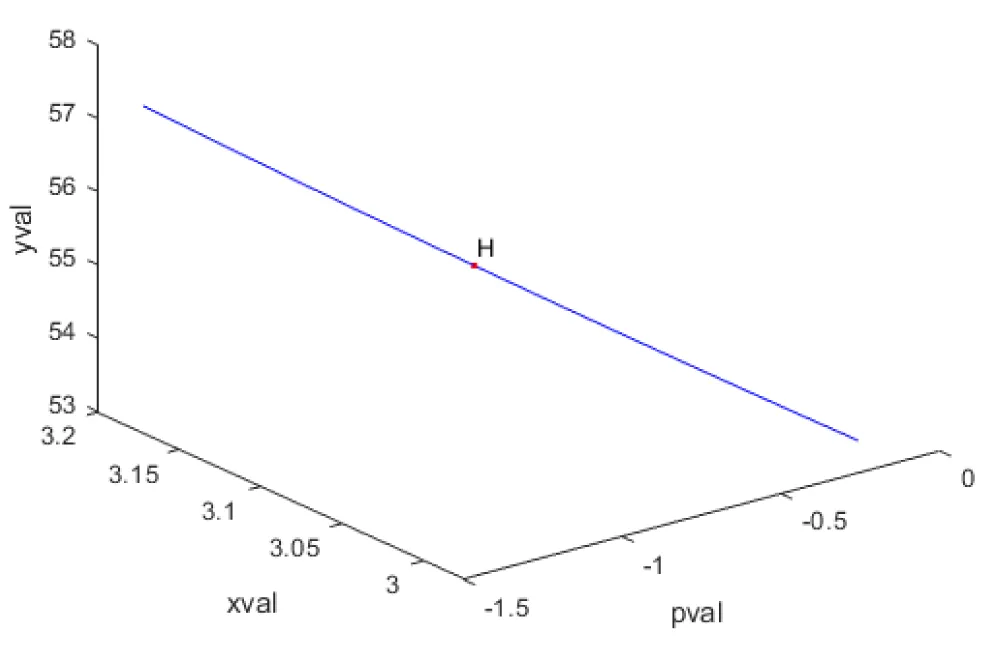
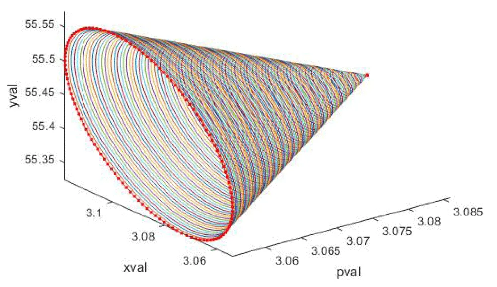
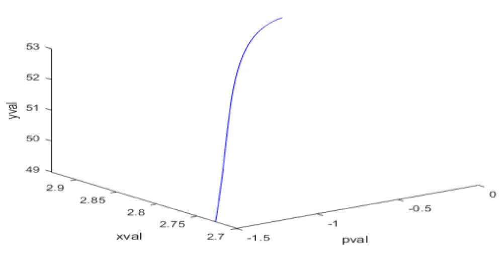
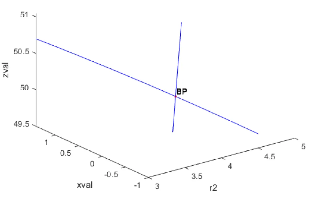
When pval was used as the bifurcation parameter, a Hopf bifurcation point was located at (xval, yval, pval) values of (3.086053, 55.448945, -0.898380). This is shown in Figure 1a. The limit cycle caused by this Hopf bifurcation point is shown in Figure 1b. When pval was changed to pval(tanh(pval)), the Hopf bifurcation point disappears, validating the analysis in Sridhar [36] where it is demonstrated with several examples that the activation factor involving the tanh function successfully eliminates the limit cycle causing Hopf bifurcation points. This is shown in Figure 1c. When r₂ was used as the bifurcation parameter, a branch point was located at

(xval, yval, r₂) values of ( 0.000000 50.049900 4.003996 ). This is shown in Figure 1d.

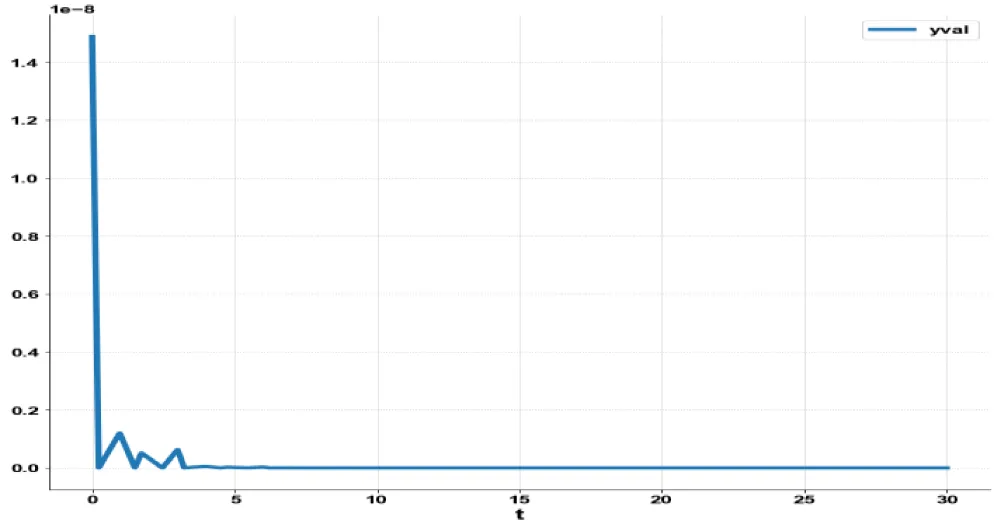
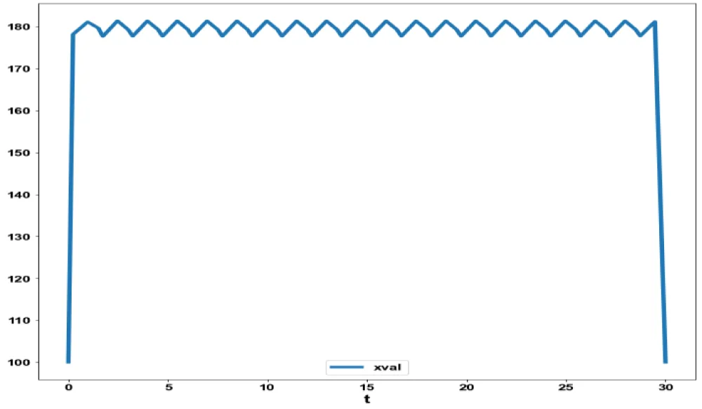
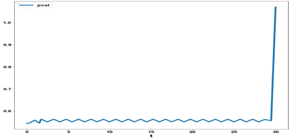
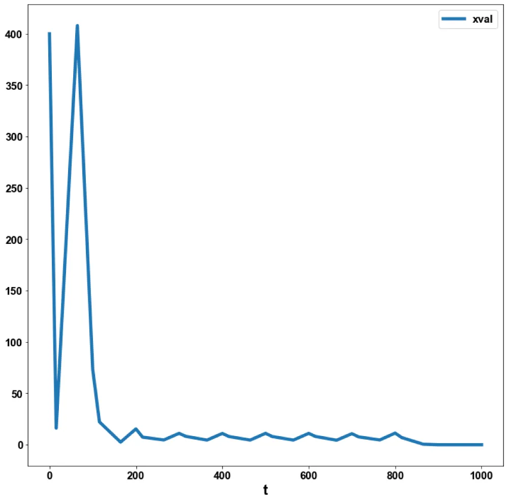
For the MNLMPC calculations, ${\displaystyle \sum _{t_{i=0}}^{t_i=t_f}xval(t_i)},{\displaystyle \sum _{t_{i=0}}^{t_i=t_f}yval(t_i)}$ were minimized individually and led to values of 200 and 0. pval was the control parameter. The multiobjective optimal control problem will involve the minimization of the subject to the equations governing Model 1. This led to a value of zero (the Utopia solution). The MNLMPC value of pval was 0.54427. Figures 1e-1g show the various MNLMPC profiles.

Model 2

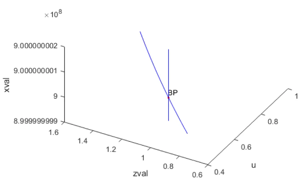
In model 2, when bifurcation analysis was performed, with u as a parameter, a branch point was located at (xval, yval, vval,zval,u) values of ( 9.e + 08, 0,0, 1.043561, 0.582576 ). This is seen in Figure 2a.

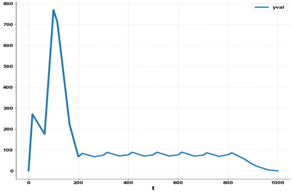
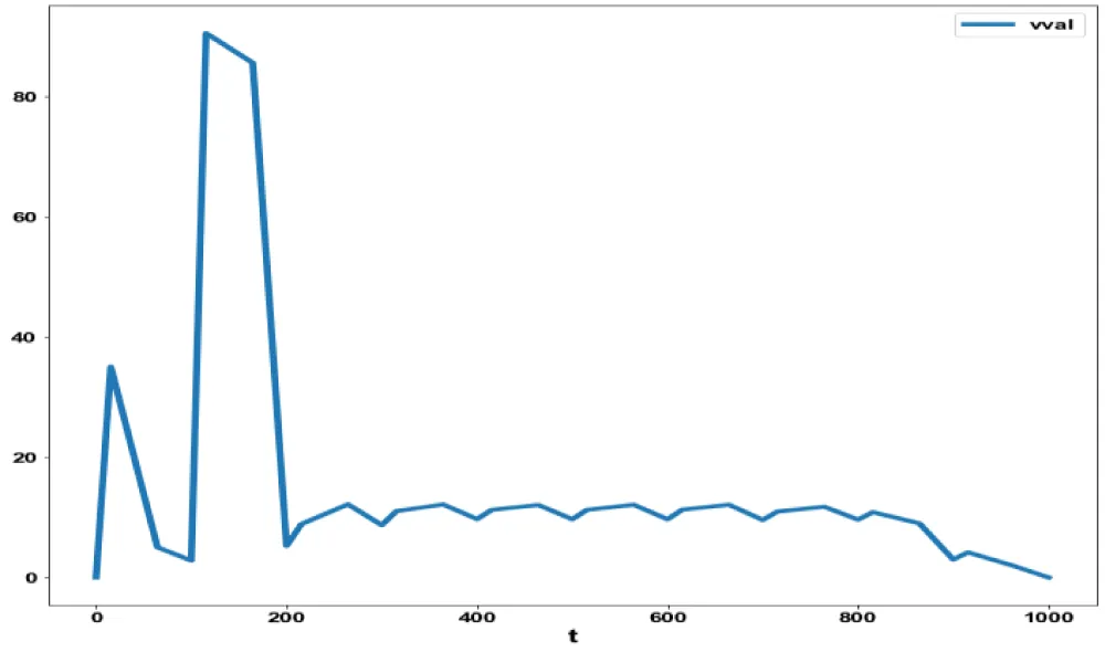
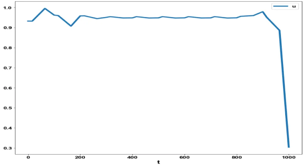
For the MNLMPC calculations, xval(0) was set as 400 and was minimized individually, yielding values of 400, 0, and 0. The multiobjective optimal control problem will involve the minimization of the ${({\displaystyle \sum _{t_{i=0}}^{t_i=t_f}xval(t_i)-400})}^2+{({\displaystyle \sum _{t_{i=0}}^{t_i=t_f}yval(t_i)}-0)}^2+{({\displaystyle \sum _{t_{i=0}}^{t_i=t_f}vval(t_i)}-0)}^2$ subject to the equations governing Model 2. This led to a value of zero (the Utopia solution). The MNLMPC value of u was 0.932. Figures 2b-2d, and 2e show the various MNLMPC profiles for Model 2.

Model 3

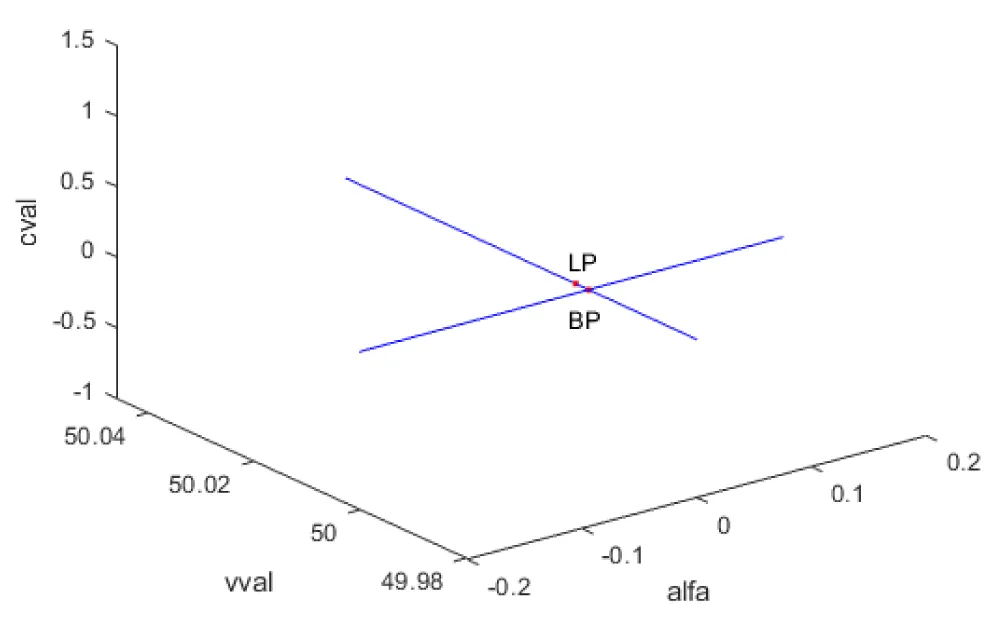
In model 3, when bifurcation analysis was performed, with as a parameter, a branch point was located at values of. (0, 50, 0, 0.119904, 0.000065). Additionally, a limit point was found at values of (0.009703, 50.002421, 0, 0.119904, 0.000065). This is shown in Figure 3a.

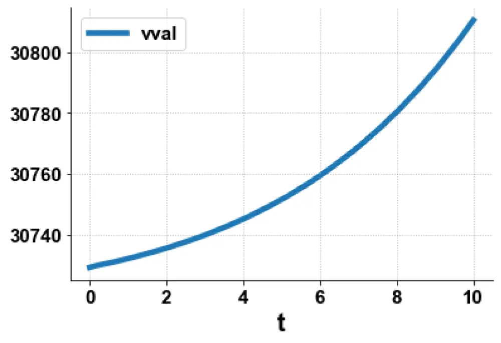
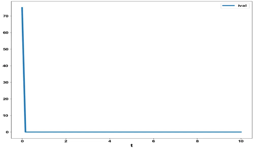
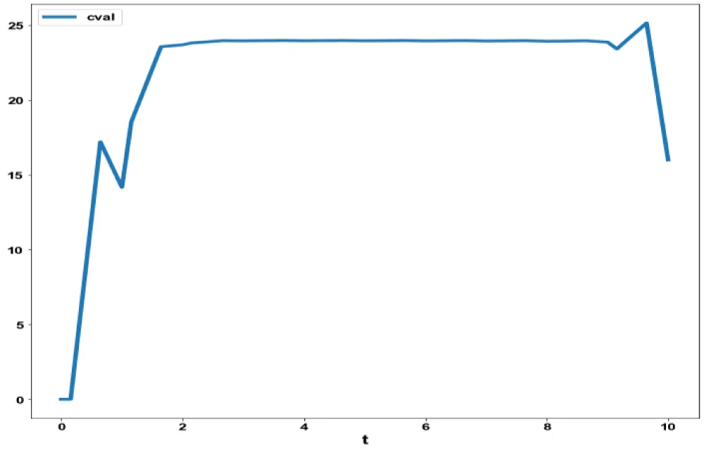
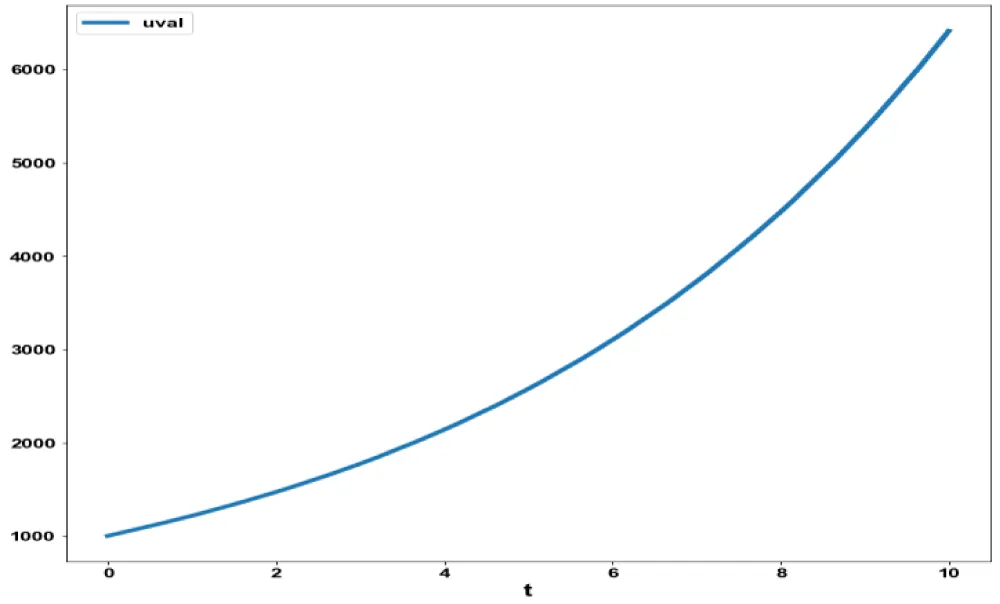
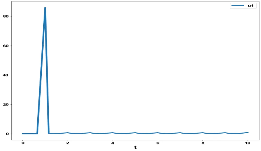
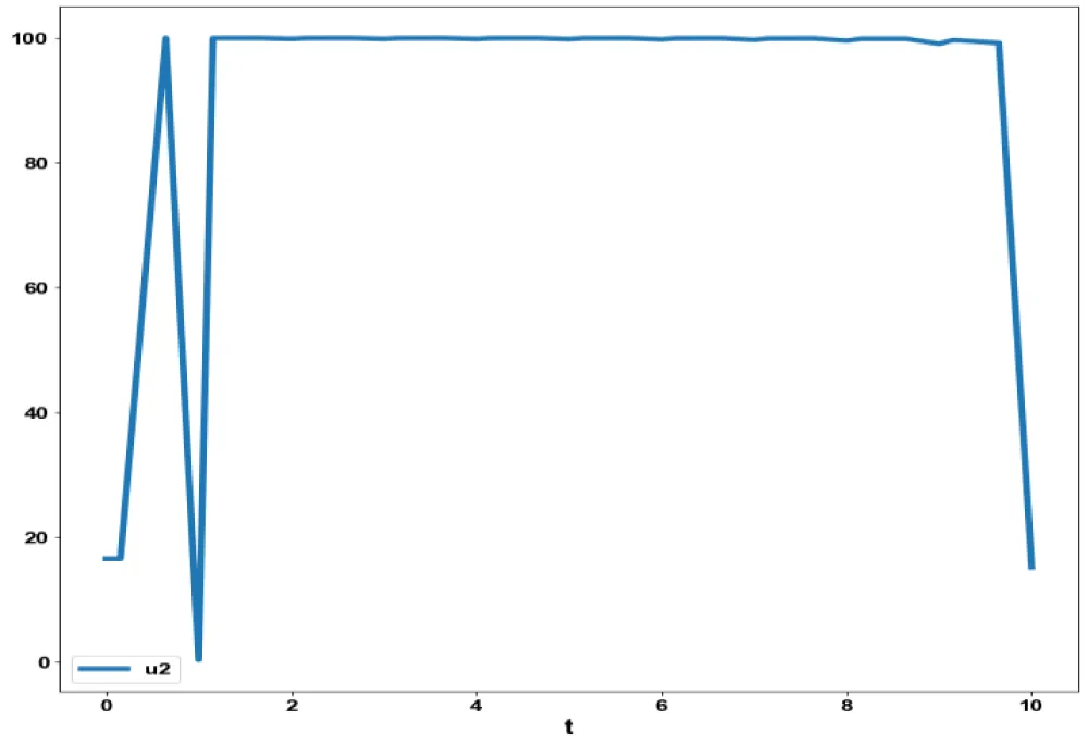
For the MNLMPC calculations, uval(0) was set as 1000, ival(0) was set as 75. They were minimized individually, yielding values of 6.1539610796052817e+04 and 75. The multiobjective optimal control problem will involve the minimization of the ${({\displaystyle \sum _{t_{i=0}}^{t_i=t_f}vval(t_i)-\text{6}\text{.1539610796052817e+04}})}^2+{({\displaystyle \sum _{t_{i=0}}^{t_i=t_f}ival(t_i)}-75)}^2$ subject to the equations governing Model 3. This led to a value of zero (the Utopia solution). The MNLMPC value of u1 and u2 (the two control parameters) were 7.863627108510299e-07 and 16.542884153050405. Figures 3b-3g show the various MNLMPC profiles for Model 3.

6. Discussion of results

Model 1 exhibits a Hopf bifurcation point, which is eliminated using an activation factor involving a tanh function, validating the analysis in Sridhar [36]. All three models exhibit branch points. These branch points enable the MNLMC calculations to yield the Utopia solution, validating the analysis in Sridhar [41]. The following paragraphs explain the cause of the occurrence of the branch points.

Theorem

If one of the functions in a dynamic system is separable into two distinct functions, a branch point singularity will occur in the system.

Proof

Consider a system of equations.

$\frac{dx}{dt}=f(x,\alpha )\text{ (15)}$

x ∈ Rn . Defining the matrix A as

$A=\left[\begin{array}{l}\frac{\partial f_1}{\partial x_1}\frac{\partial f_1}{\partial x_2}\frac{\partial f_1}{\partial x_3}\frac{\partial f_1}{\partial x_4}\mathrm{..........}\frac{\partial f_1}{\partial x_n}\frac{\partial f_1}{\partial \alpha }\\ \frac{\partial f_2}{\partial x_1}\frac{\partial f_2}{\partial x_2}\frac{\partial f_2}{\partial x_3}\frac{\partial f_2}{\partial x_4}\mathrm{..........}\frac{\partial f_2}{\partial x_n}\frac{\partial f_2}{\partial \alpha }\\ \mathrm{...........................................................}\\ \mathrm{...........................................................}\\ \frac{\partial f_n}{\partial x_1}\frac{\partial f_n}{\partial x_2}\frac{\partial f_n}{\partial x_3}\frac{\partial f_n}{\partial x_4}\mathrm{..........}\frac{\partial f_n}{\partial x_n}\frac{\partial f_n}{\partial \alpha }\end{array}\right]\text{ (16)}$

α Is the bifurcation parameter. The matrix A can be written in a compact form as

$A=[\frac{\partial f_p}{\partial x_q}.|\frac{\partial f_p}{\partial \alpha }]\text{ (17)}$

The tangent at any point x; ( $z=[z_1,z_2,z_3,z_4,\mathrm{....}{z}_{n+1}]$ ) must satisfy

$Az=0\text{ (18)}$

The matrix must be singular at both limit and branch points. The n+1th component of the tangent vector Z_n+1 = 0 at a limit point (LP), and for a branch point (BP), the matrix must be singular.

Any tangent at a point y that is defined by $z=[z_1,z_2,z_3,z_4,\mathrm{....}{z}_{n+1}]$ ) must satisfy.

$Az=0\text{ (19)}$

For a branch point, there must exist two tangents at the singularity. Let the two tangents be z and w. This implies that

$\begin{array}{l}Az=0\\ Aw=0\text{ (20)}\end{array}$

Consider a vector v that is orthogonal to one of the tangents (say z). v can be expressed as a linear combination of z and w ( $v=\alpha z+\beta w$ ). Since z and v are orthogonal,

$z^{T}v=0$ . Hence, this implies that B is singular.

Let any of the functions f_i be separable into 2 functions ${\varphi }_1,{\varphi }_2$ as

$f_i={\varphi }_1{\varphi }_2\text{ (21)}$

At steady-state $f_i(x,\alpha )=0$ and this will imply that either or both must be 0. This implies that the two branches will meet at a point where both are 0.

At this point, the matrix B will be singular, as a row in this matrix would be

$[\frac{\partial f_i}{\partial x_k}|\frac{\partial f_i}{\partial \alpha }]\text{ (22)}$

However,

$\begin{array}{l}[\frac{\partial f_i}{\partial x_k}={\varphi }_1(=0)\frac{\partial {\varphi }_2}{\partial x_k}+{\varphi }_2(=0)\frac{\partial {\varphi }_1}{\partial x_k}=0(\forall k=1.,,n)\text{ (23)}\\ \frac{\partial f_i}{\partial \alpha }={\varphi }_1(=0)\frac{\partial {\varphi }_2}{\partial \alpha }+{\varphi }_2(=0)\frac{\partial {\varphi }_1}{\partial \alpha }]=0\end{array}$

This implies that every element in the row would be 0, and hence the matrix B would be singular. The singularity in B implies that there exists a branch point.

In model 1, a branch point was located at

(xval, yval) values of ( 0.000000 50.049900 ). Here, the two distinct functions can be obtained from the first equation in Model 1

$\frac{d(xval)}{dt}=r_1(xval)(1-\frac{(pval(xval)+qval(yval))}{k})-\frac{b(xval)yval}{\left(xval+yval+a\right)}.\text{ (24)}$

The 2 distinct function branches are

$xval=0\text{ (25)}$

and

$r_1(1-\frac{(pval(xval)+qval(yval))}{k})-\frac{b(yval)}{\left(xval+yval+a\right)}=0\text{ (26)}$

The values satisfy both the above equations, confirming the correctness of the theorem.

In model 2, a branch point was located at (xval, yval, vval,zval,u) values of ( 9.e+08; 0;0; 1 .043561 0.582576 ). The two distinct functions can be seen from the second equation of Model 2,

$\frac{d(yval)}{dt}=\left(\frac{\beta (xval)yval(zval)}{\left(xval+yval+\epsilon \right)}\right)-\left(1-u\right)\delta yval\text{ (27)}$

Here, the two distinct function branches are

$yval=0\text{ (28)}$

and

$\left(\frac{\beta (xval)(zval)}{\left(xval+yval+\epsilon \right)}\right)-\left(1-u\right)\delta \text{ (29)}$

Substituting $\beta =0.2;\epsilon =0.009;\delta =0.5;xval=9.0e+08;zval=1.043561\text{ u=}0.582576yval=0;$

Satisfies both the above equations, confirming the correctness of the theorem.

In model 3, a branch point was located at values of. (0, 50, 0, 0.119904, 0.000065) and the two distinct branches can be obtained from the first equation in model 3, which is

$\frac{d(uval)}{dt}=\alpha (uval)\left(1- \left(\frac{\left(uval+ival\right)}{k}\right)\right)-\left(\frac{\beta (uval)vval}{ku+uval}\right)-\left(\frac{{\delta }_u(uval)cval}{\left(kc+cval\right)}\right)\text{ (30)}$

These 2 branches are

$uval=0\text{ (31)}$

and

$\alpha \left(1- \left(\frac{\left(uval+ival\right)}{k}\right)\right)-\left(\frac{\beta vval}{ku+uval}\right)-\left(\frac{{\delta }_{u}cval}{\left(kc+cval\right)}\right)=0\text{ (32)}$

Substituting $\begin{array}{l}k=1.e+06;\beta =0.01;{\delta }_u=50;ku=1.e+05;kc=1.e+05;\\ \text{uval=}0,\text{ vval=}50,\text{ ival=}0,\text{ cval=}0.119904,\alpha =0.000065\end{array}$

Satisfies both the above equations, confirming the correctness of the theorem.

Conclusion

Bifurcation analysis and multiobjective nonlinear control (MNLMPC) studies in three oncolytic virus models. The bifurcation analysis revealed the existence of a Hopf bifurcation point in one of the models and branch points in all three models. The Hopf bifurcation point was eliminated using an activation factor that involves the tanh function. The branch points (which cause multiple steady-state solutions from a singular point) are very beneficial because they enable the Multiobjective nonlinear model predictive control calculations to converge to the Utopia point (the best possible solution) in the models. It is proven (with computational validation) that the branch points were caused because of the existence of two distinct separable functions in one of the equations in each dynamic model. A theorem was developed to demonstrate this fact for any dynamic model. A combination of bifurcation analysis and Multiobjective Nonlinear Model Predictive Control(MNLMPC) for dynamic models involving oncolytic viral therapy is the main contribution of this paper.

Data availability statement

All data used is presented in the paper

Conflict of interest

The author, Dr. Lakshmi N Sridhar, has no conflict of interest.

Dr. Sridhar thanks Dr. Carlos Ramirez and Dr. Suleiman for encouraging him to write single-author papers.

1. Mullen JT, Tanabe KK. Viral oncolysis. Oncologist. 2002;7(2):106-19. Available from: https://doi.org/10.1634/theoncologist.7-2-106
2. Chiocca EA. Oncolytic viruses. Nat Rev Cancer. 2002;2(12):938-50. Available from: https://doi.org/10.1158/2326-6066.cir-14-0015
3. Aghi M, Martuza RL. Oncolytic viral therapies - the clinical experience. Oncogene. 2005;24(52):7802-16. Available from: https://doi.org/10.1038/sj.onc.1209037
4. Novozhilov AS, Berezovskaya FS, Koonin EV, Karev GP. Mathematical modeling of tumor therapy with oncolytic viruses: regimes with complete tumor elimination within the framework of deterministic models. Biol Direct. 2006;1:6. Available from: https://doi.org/10.1186/1745-6150-1-6
5. Kelly E, Russell SJ. History of oncolytic viruses: genesis to genetic engineering. Mol Ther. 2007;15(4):651-9. Available from: https://doi.org/10.1038/sj.mt.6300108
6. Alonso M, Gomez-Manzano C, Jiang H, Bekele NB, Piao Y, Yung WKA, et al. Combination of the oncolytic adenovirus ICOVIR-5 with chemotherapy provides enhanced anti-glioma effect in vivo. Cancer Gene Ther. 2007;14:756–61. Available from: https://doi.org/10.1038/sj.cgt.7701067
7. Zurakowski R, Wodarz D. Model-driven approaches for in vitro combination therapy using ONYX-015 replicating oncolytic adenovirus. J Theor Biol. 2007;245(1):1–8. Available from: https://doi.org/10.1016/j.jtbi.2006.09.029
8. Wong HH, Lemoine N, Wang Y. Oncolytic viruses for cancer therapy: overcoming the obstacles. Viruses. 2010;2(1):78–106. Available from: https://doi.org/10.3390/v2010078
9. Ottolino PK, Diallo JS, Lichty BD, Bell JC, McCart JA. Intelligent design: combination therapy with oncolytic viruses. Mol Ther. 2010;18:251–63. Available from: https://doi.org/10.1038/mt.2009.283
10. Komarova NL, Wodarz D. ODE models for oncolytic virus dynamics. J Theor Biol. 2010;263(4):530–43. Available from: https://doi.org/10.1016/j.jtbi.2010.01.009
11. Eager RM, Nemunaitis J. Clinical development directions in oncolytic viral therapy. Cancer Gene Ther. 2011;18(5):305–17. Available from: https://www.nature.com/articles/cgt20117
12. Agarwal M, Bhadauria AS. Mathematical modelling and analysis of tumor therapy with oncolytic virus. Appl Math. 2011;2(1):131–40. Available from: https://www.scirp.org/journal/paperinformation?paperid=3819
13. Bagheri N, Shiina M, Lauffenburger DA, Korn WM. A dynamical systems model for combinatorial cancer therapy enhances oncolytic adenovirus efficacy by MEK-inhibition. PLoS Comput Biol. 2011;7(2):e1001085. Available from: https://doi.org/10.1371/journal.pcbi.1001085
14. Tian JP. The replicability of oncolytic virus: defining conditions in tumor virotherapy. Math Biosci Eng. 2011;8:841–60. Available from: https://doi.org/10.3934/mbe.2011.8.841
15. Donnelly OG, Errington-Mais F, Prestwich R, Harrington K, Pandha H, Vile R, et al. Recent clinical experience with oncolytic viruses. Curr Pharm Biotechnol. 2012;13(9):1834–41. Available from: https://doi.org/10.2174/138920112800958904
16. Russell SJ, Peng KW, Bell JC. Oncolytic virotherapy. Nat Biotechnol. 2012;30(7):658–70. Available from: https://doi.org/10.1038/nbt.2287
17. Zhou L, He WW, Zhu ZN. The clinical research progress for oncolytic adenovirus targeting cancer therapy. China Biotechnol. 2013;33(12):105–13.
18. Patel MR, Kratzke RA. Oncolytic virus therapy for cancer: the first wave of translational clinical trials. Transl Res. 2013;161(4):355–64. Available from: https://doi.org/10.1016/j.trsl.2012.12.010
19. Wang Y, Tian JP, Wei J. Lytic cycle: a defining process in oncolytic virotherapy. Appl Math Model. 2013;37(8):5962–78. Available from: https://doi.org/10.1016/j.apm.2012.12.004
20. Kim PS, Crivelli JJ, Choi IK, Yun CO, Wares JR. Quantitative impact of immunomodulation versus oncolysis with cytokine-expressing virus therapeutic. Math Biosci Eng. 2015;12(4):841–58. Available from: https://doi.org/10.3934/mbe.2015.12.841
21. Si W, Zhang W. Control exponential growth of tumor cells with slow spread of oncolytic virus. J Theor Biol. 2015;367:111–29. Available from: https://doi.org/10.1016/j.jtbi.2014.11.015
22. Chen Y, Su YM. An improved model of tumor therapy with oncolytic virus. J Henan Univ Sci Technol. 2016;37(4):92–6.
23. Simpson GR, Relph K, Harrington K, Melcher A, Pandha H. Cancer immunotherapy via combining oncolytic virotherapy with chemotherapy: recent advances. Oncolytic Virother. 2016;5:1–13. Available from: https://doi.org/10.2147/ov.s66083
24. Su Y, Jia C, Chen Y. Optimal control model of tumor treatment with oncolytic virus and MEK inhibitor. Biomed Res Int. 2016;2016:5621313. Available from: https://doi.org/10.1155/2016/5621313
25. Malinzi J, Ouifki R, Eladdadi A, Torres DFM, White JKA. Enhancement of chemotherapy using oncolytic virotherapy: mathematical and optimal control analysis. Math Biosci Eng. 2018;15(6):1435–63. Available from: https://doi.org/10.3934/mbe.2018066
26. Adi-Kusumo F, Aryati L, Risdayati S, Norhidayah S. Hopf bifurcation on a cancer therapy model by oncolytic virus involving the malignancy effect and therapeutic efficacy. Int J Math Math Sci. 2020;2020(1):4730715. Available from: https://doi.org/10.1155/2020/4730715
27. Dhooge A, Govaerts W, Kuznetsov AY. MATCONT: A Matlab package for numerical bifurcation analysis of ODEs. ACM Trans Math Softw. 2003;29(2):141–64. Available from: https://lab.semi.ac.cn/download/0.28315849875964405.pdf
28. Dhooge A, Govaerts W, Kuznetsov YA, Mestrom W, Riet AM. CL_MATCONT: A continuation toolbox in Matlab. 2004. Available from: https://doi.org/10.1145/952532.952567
29. Kuznetsov YA. Elements of applied bifurcation theory. New York: Springer; 1998. Available from: https://www.ma.imperial.ac.uk/~dturaev/kuznetsov.pdf
30. Kuznetsov YA. Five lectures on numerical bifurcation analysis. Utrecht University; 2009.
31. Govaerts WJF. Numerical methods for bifurcations of dynamical equilibria. Philadelphia: SIAM; 2000. Available from: https://epubs.siam.org/doi/pdf/10.1137/1.9780898719543.fm
32. Dubey SR, Singh SK, Chaudhuri BB. Activation functions in deep learning: a comprehensive survey and benchmark. Neurocomputing. 2022;503:92–108. Available from: https://doi.org/10.1016/j.neucom.2022.06.111
33. Kamalov AF, Nazir M, Safaraliev AK, Cherukuri, Zgheib R. Comparative analysis of activation functions in neural networks. In: 2021 28th IEEE International Conference on Electronics, Circuits, and Systems (ICECS); 2021; Dubai, United Arab Emirates. p. 1–6. Available from: https://ieeexplore.ieee.org/document/9665646
34. Szandała T. Review and comparison of commonly used activation functions for deep neural networks. ArXiv. 2020:203–24. Available from: https://link.springer.com/chapter/10.1007/978-981-15-5495-7_11
35. Sridhar LN. Bifurcation analysis and optimal control of the tumor macrophage interactions. Biomed J Sci Tech Res. 2023;53(5):45218–25. Available from: https://ideas.repec.org/a/abf/journl/v53y2023i5p45218-45225.html
36. Sridhar LN. Elimination of oscillation causing Hopf bifurcations in engineering problems. J Appl Math. 2024;2(4):1826. Available from: https://ojs.acad-pub.com/index.php/JAM/article/view/1826
37. Flores-Tlacuahuac A, Morales P, Riveral Toledo M. Multiobjective nonlinear model predictive control of a class of chemical reactors. Ind Eng Chem Res. 2012;51:5891–9. Available from: https://pubs.acs.org/doi/abs/10.1021/ie201742e
38. Hart WE, Laird CD, Watson JP, Woodruff DL, Hackebeil GA, Nicholson BL, et al. Pyomo – Optimization modeling in Python. 2nd ed. Vol. 67. Available from: https://link.springer.com/book/10.1007/978-3-030-68928-5
39. Wächter A, Biegler L. On the implementation of an interior-point filter line-search algorithm for large-scale nonlinear programming. Math Program. 2006;106:25–57. Available from: https://doi.org/10.1007/s10107-004-0559-y
40. Tawarmalani M, Sahinidis NV. A polyhedral branch-and-cut approach to global optimization. Math Program. 2005;103(2):225–49. Available from: https://link.springer.com/article/10.1007/s10107-005-0581-8
41. Sridhar LN. Coupling bifurcation analysis and multiobjective nonlinear model predictive control. Austin Chem Eng. 2024;10(3):1107. Available from: https://austinpublishinggroup.com/chemical-engineering/fulltext/ace-v11-id1107.pdf
42.  Upreti SR. Optimal control for chemical engineers. Boca Raton (FL): Taylor & Francis; 2013.